MDNs take your boring old neural network and turn it into a prediction powerhouse. Why settle for just one prediction when you can have a whole buffet of potential outcomes?

The basic idea
In an MDN, the probability density of the target variable t given the entry X is represented as a linear combination of kernel functions, usually Gaussian functions, but not limited to them. In mathematics, speak:

Where 𝛼ᵢ(x) are the mixing coefficients, and who doesn't love a good mixing, right? 🎛️ These determine how much weight each component 𝜙ᵢ(t|x) — every Gaussian in our case is valid in the model.
Mix the Gaussians ☕
Each Gaussian component 𝜙ᵢ(t|x) has its own mean 𝜇ᵢ(x) and variance 𝜎ᵢ².

Mix 🎧 with coefficients
The mixing coefficients 𝛼ᵢ are crucial because they balance the influence of each Gaussian component, governed by a softmax function to make sure they add up to 1:

Magic Parameters ✨ Averages and deviations
Means 𝜇ᵢ and deviations 𝜎ᵢ² define each Gaussian. And guess what? The differences must be positive! We achieve this by using the exponential of the network outputs:

Okay, so how do we train this beast? Well, it's about maximizing the probability of our observed data. Fancy terms, I know. Let's see it in action.
The fate of log-likelihood ✨
The probability of our data under the MDN model is the product of the probabilities assigned to each data point. In mathematics, speak:

This basically says, “Hey, what’s the chance we have this data given our model?”. But products can get complicated, so we take the newspaper (because math loves newspapers), which turns our product into a sum:

Now here's the thing: we actually want to minimize the probability of negative logging because our optimization algorithms like to minimize things. So, plugging in the definition of p(t|x)the error function that we actually minimize is:

This formula may seem intimidating, but it simply says that we summarize the log probabilities for all data points and then add a negative sign, because minimization is our problem.
Now here's how to translate our magic into Python, and you can find the full code here:
The loss function
def mdn_loss(alpha, sigma, mu, target, eps=1e-8):
target = target.unsqueeze(1).expand_as(mu)
m = torch.distributions.Normal(loc=mu, scale=sigma)
log_prob = m.log_prob(target)
log_prob = log_prob.sum(dim=2)
log_alpha = torch.log(alpha + eps)  # Avoid log(0) disaster
loss = -torch.logsumexp(log_alpha + log_prob, dim=1)
return loss.mean()
Here is the breakdown:
target = target.unsqueeze(1).expand_as(mu): Enlarge the target to match the shape ofmu.m = torch.distributions.Normal(loc=mu, scale=sigma): Create a normal distribution.log_prob = m.log_prob(target): Calculate the logarithmic probability.log_prob = log_prob.sum(dim=2): Sum of log probabilities.log_alpha = torch.log(alpha + eps): Calculate the log of mixing coefficients.loss = -torch.logsumexp(log_alpha + log_prob, dim=1): Combine and record the sum of the probabilities.return loss.mean(): Returns the average loss.
The neural network
Let's create a neural network ready to handle magic:
class MDN(nn.Module):
def __init__(self, input_dim, output_dim, num_hidden, num_mixtures):
super(MDN, self).__init__()
self.hidden = nn.Sequential(
nn.Linear(input_dim, num_hidden),
nn.Tanh(),
nn.Linear(num_hidden, num_hidden),
nn.Tanh(),
)
self.z_alpha = nn.Linear(num_hidden, num_mixtures)
self.z_sigma = nn.Linear(num_hidden, num_mixtures * output_dim)
self.z_mu = nn.Linear(num_hidden, num_mixtures * output_dim)
self.num_mixtures = num_mixtures
self.output_dim = output_dimdef forward(self, x):
hidden = self.hidden(x)
alpha = F.softmax(self.z_alpha(hidden), dim=-1)
sigma = torch.exp(self.z_sigma(hidden)).view(-1, self.num_mixtures, self.output_dim)
mu = self.z_mu(hidden).view(-1, self.num_mixtures, self.output_dim)
return alpha, sigma, mu
Notice the softmax being applied to 𝛼ᵢ alpha = F.softmax(self.z_alpha(hidden), dim=-1)so their sum is equal to 1, and the exponential is equal to 𝜎ᵢ sigma = torch.exp(self.z_sigma(hidden)).view(-1, self.num_mixtures, self.output_dim)to ensure they remain positive, as explained previously.
The prediction
Getting predictions from MDNs is a bit of a trick. Here's how to sample from the mixture model:
def get_sample_preds(alpha, sigma, mu, samples=10):
N, K, T = mu.shape
sampled_preds = torch.zeros(N, samples, T)
uniform_samples = torch.rand(N, samples)
cum_alpha = alpha.cumsum(dim=1)
for i, j in itertools.product(range(N), range(samples)):
u = uniform_samples(i, j)
k = torch.searchsorted(cum_alpha(i), u).item()
sampled_preds(i, j) = torch.normal(mu(i, k), sigma(i, k))
return sampled_preds
Here is the breakdown:
N, K, T = mu.shape: Get the number of data points, mixture components, and output dimensions.sampled_preds = torch.zeros(N, samples, T): Initialize the tensor to store the sampled predictions.uniform_samples = torch.rand(N, samples): Generate uniform random numbers for sampling.cum_alpha = alpha.cumsum(dim=1): Calculate the cumulative sum of the weights of the mixture.for i, j in itertools.product(range(N), range(samples)): loop over each combination of data points and samples.u = uniform_samples(i, j): Get a random number for the current sample.k = torch.searchsorted(cum_alpha(i), u).item(): Find the index of the components of the mixture.sampled_preds(i, j) = torch.normal(mu(i, k), sigma(i, k)): Sample of the selected Gaussian component.return sampled_preds: Returns the tensor of the sampled predictions.
Let's apply MDN to predict “Apparent temperature” using a simple Weather dataset. I trained an MDN with a 50 hidden layer network, and guess what? It rocks ! 🎸
Find the complete code here. Here are some results: